Project 5A - Introduction

In this project, we use the DeepFloyd IF diffusion model, a two-stage model that first generates 64x64 images, then 256x256 images. In this project, I will iteratively show the different aspects of building a diffusion model.

In this project, I will use a seed of 180.

Sampling Images

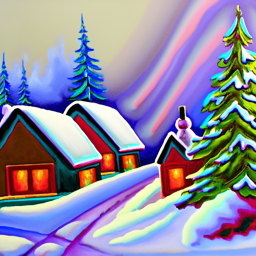
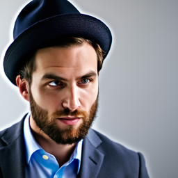
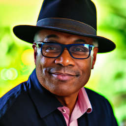
First, let's play around with the model and generate some sample images with varying num_inference_steps.

“an oil painting of a snowy mountain village”

num_inference_steps=2

“a man wearing a hat”

num_inference_steps=20

1. The oil painting of a snow mountain village displays multiple houses with snow-covered roofs and streets, but the model struggles to generate anything valuable in the top right corner. I believe it was trying to display a mountain but failed.

2. For the middle image of a man wearing a hat, the model successfully generates a man wearing a hat but messes up the direction of the man's eyes, so it looks a bit silly. Below, I generated an image with num_inference_steps=40, and the output is noticeably better, as the picture looks much more realistic.

3. For the final image, the model successfully generates a rocket ship blasting off from space, drawing a cloud and its flume trail. However, the generated image looks a bit too "cartoon-y" and not very realistic. Below, I ran the same prompt with num_inference_steps=40. I would've expected a noticeable increase in quality since I doubled the num_inference_steps, but the output doesn't look much better. As you can see, increasing the number of inference steps does not always lead to an improvement in the model's output.

“a man wearing a hat”

num_inference_steps=40

“a rocket ship”

num_inference_steps=40

Sampling Loops

In this part of the problem set, I will write my own "sampling loops" that use the pre-trained DeepFloyd denoisers that should produce high-quality images such as the ones generated above.

I will also modify these sampling loops to solve different tasks, such as inpainting or producing optical illusions.

In the examples below, I will use the following image of UC Berkeley's clocktower, the "Campanile,” as an example image.

1.1 Implementing the Forward Process

In this part, I implement the forward process of a diffusion model, which takes in an image and iteratively adds more noise to the image based on the timestep t. In my implementation, t ranges from 0 to 999. To enable this functionality, I wrote a function defined as forward(img,t), which implements the following equations:

$q(x_t | x_0) = \mathcal{N}(x_t; \sqrt{\bar{\alpha}_t} x_0, (1 - \bar{\alpha}_t) \mathbf{I})$

which is equivalent to:

$x_t = \sqrt{\bar{\alpha}_t} x_0 + \sqrt{1 - \bar{\alpha}_t} \, \epsilon \quad \text{where} \quad \epsilon \sim \mathcal{N}(0, 1)$

After applying the sample image to the forward process with varying values of t, I got the following results:

t = 0

t = 250

t=500

t=750

t=999

1.2 Classical Denoising

Let's try reverting the results of the forward process to get the original image, where t = [250, 500, 750]. To do this, we will use a Gaussian blur with varying sigma values.

Note that for each sigma, I set the kernel_size to be ksize = int(3 * sigma + 1), adding 1 if ksize was even to ensure ksize is odd.

Here are my results:

Forward w/ t=250

Blurred w/ sigma=0.75

Forward w/ t=500

Forward w/ t=750

Blurred w/ sigma=0.75

Blurred w/ sigma=3

1.3 Implementing One-Step Denoising

Now, let's use a pre-trained diffusion model to denoise. To do this, we will use a U-net to recover the Gaussian noise in an image, conditioned on the timestep t. Since the diffusion model was trained on text conditioning, I use the embedding of the prompt "a high quality photo" to condition the model.

Here are my results:

Forward w/ t=250

Estimate for t=250

Forward w/ t=500

Forward w/ t=750

Estimate for t=500

Estimate for t=750

1.4 Implementing Iterative Denoising

Next, we'll implement iterative denoising. To accomplish this, we will predict the image at thet' timestep where t'=timestep[i_start + 1]. This is done by implementing the following equation in a function called iterative_denoise(image, i_start):

$x_{t'} = \frac{\sqrt{\bar{\alpha}_{t'} \beta_t}}{1 - \bar{\alpha}_t} x_0 + \frac{\sqrt{\alpha_t (1 - \bar{\alpha}_{t'})}}{1 - \bar{\alpha}_t} x_t + v_\sigma$

This starts the denoising process at t = timestep[i_start] instead of t=999.

Below, I show the denoising process.

t=690

t=540

t=390

t=240

t=90

Here is the result of the denoising process:

Here is the result of the clean one-step denoising from the section above:

Here is the blurred-noisy image, where I apply a Gaussian blur with sigma=2 and ksize=5 to the result of the test_image after the forward process.

1.5 Diffusion Model Sampling

In this part, I generate a random noisy tensor of shape (1, 3, 64, 64) and pass it to the diffusion model where the conditional embedding is the embedding of "a high quality photo” and i_start=0.

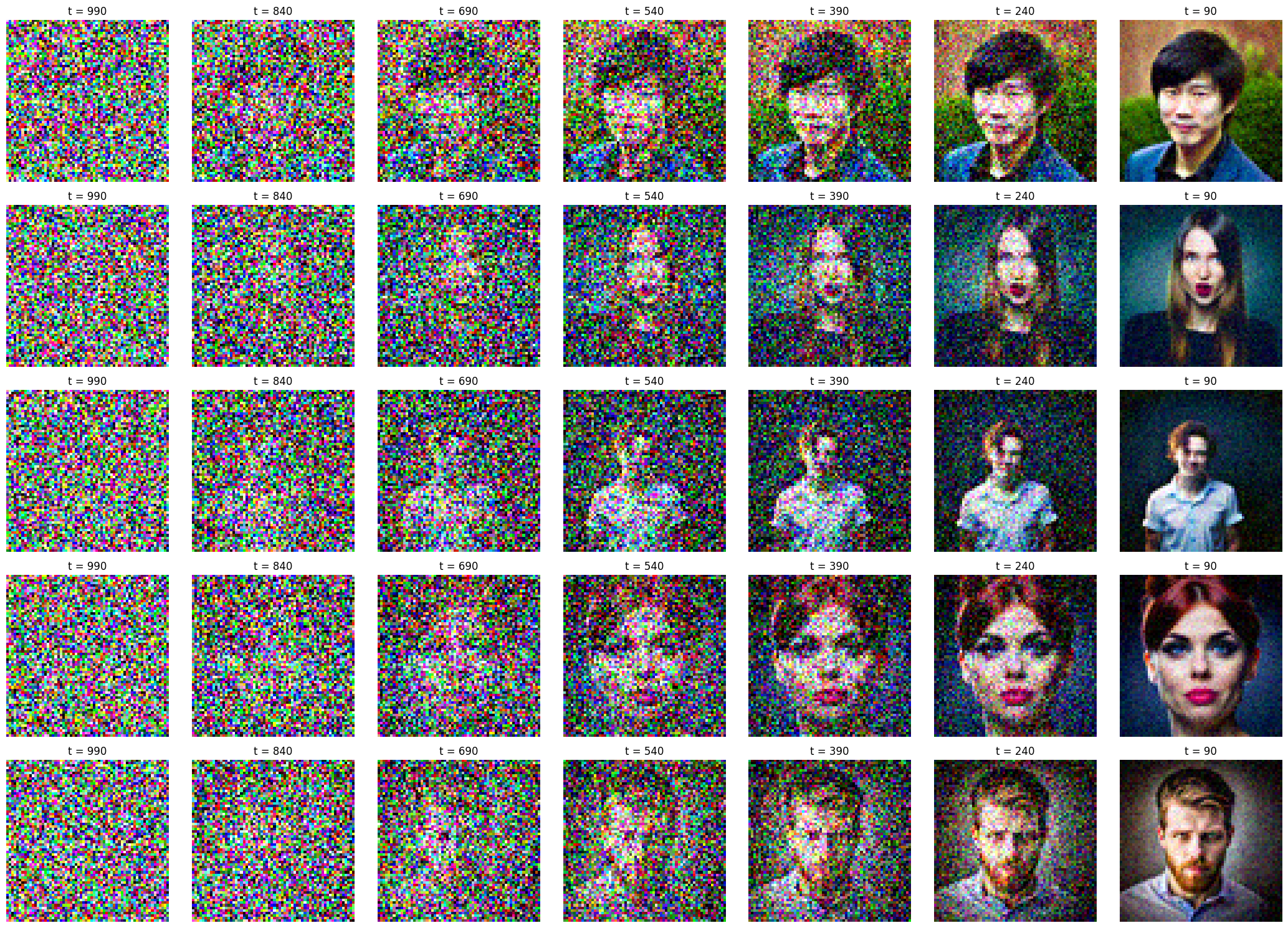
Here are five images generated using this process:

1.6 Classifier Free Guidance

In the previous part (1.5), you may have noticed that the model generated images have poor quality. To solve this, we use Classifier Free Guidance, an algorithm that takes a linear combination of unconditional and conditional noise based on a constant $\gamma$.

$\epsilon = \epsilon_u + \gamma (\epsilon_c - \epsilon_u)$

When $\gamma > 1$, generated images have very high quality output. The noise are the results of passing the image through a model that applies the conditional text embedding of prompt "a high quality photo" and unconditional text embedding of prompt "".

Here are five images generated using this process where I set $\gamma=7$

1.7 Image-to-Image Translation

In this part, we will add noise to a test image by running it through the forward function, then pass the noisy test image to our model for de-noising. As you will see, the more noisy the test image, the more the model hallucinates.

To demonstrate this, I will generate images with varying the strided-timestep index I start at from [1, 3, 5, 7, 10, 20]. In the image below, the first progression is i_start=1 and the final progression is i_start=20.

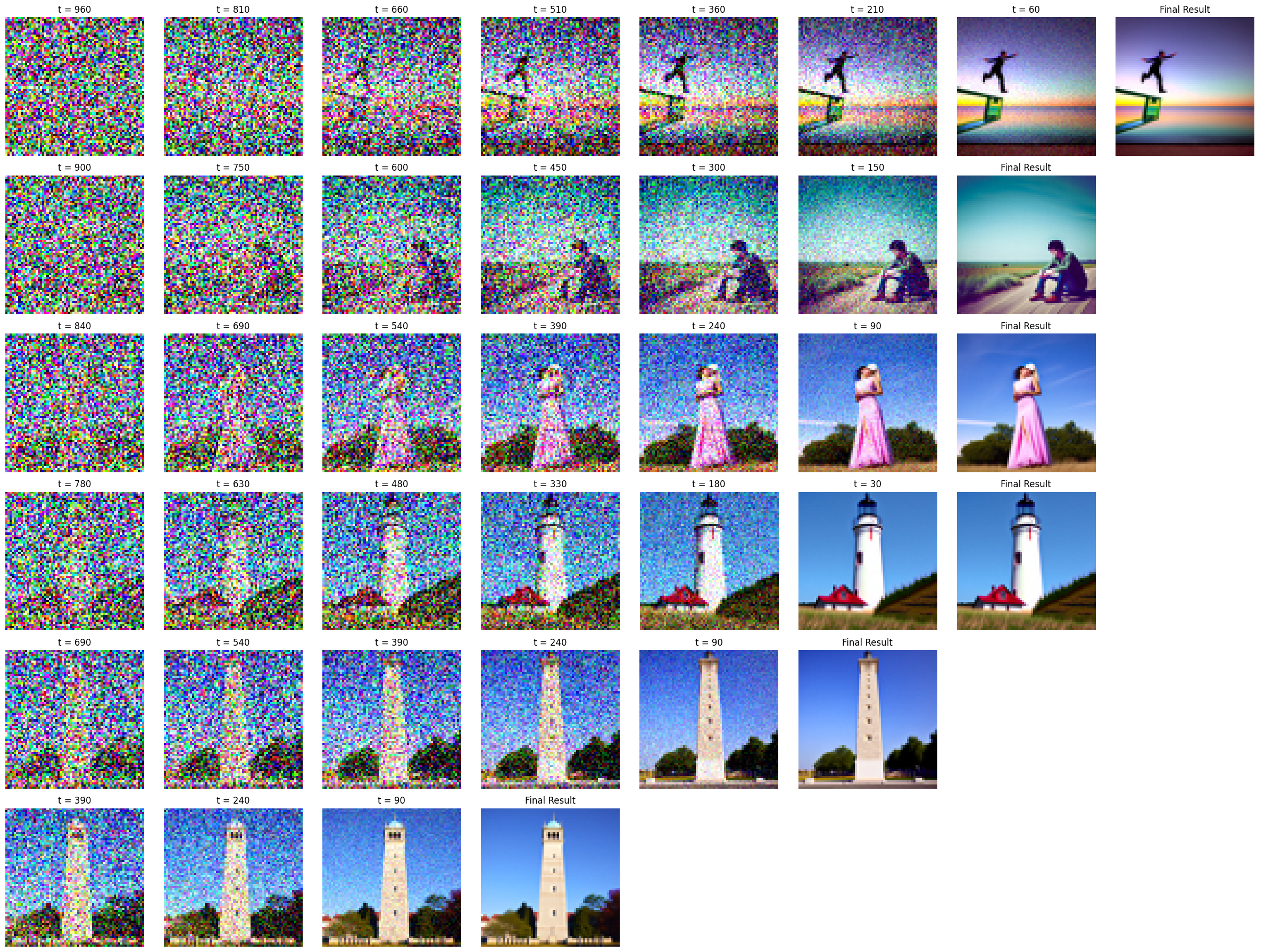
Here are my results:

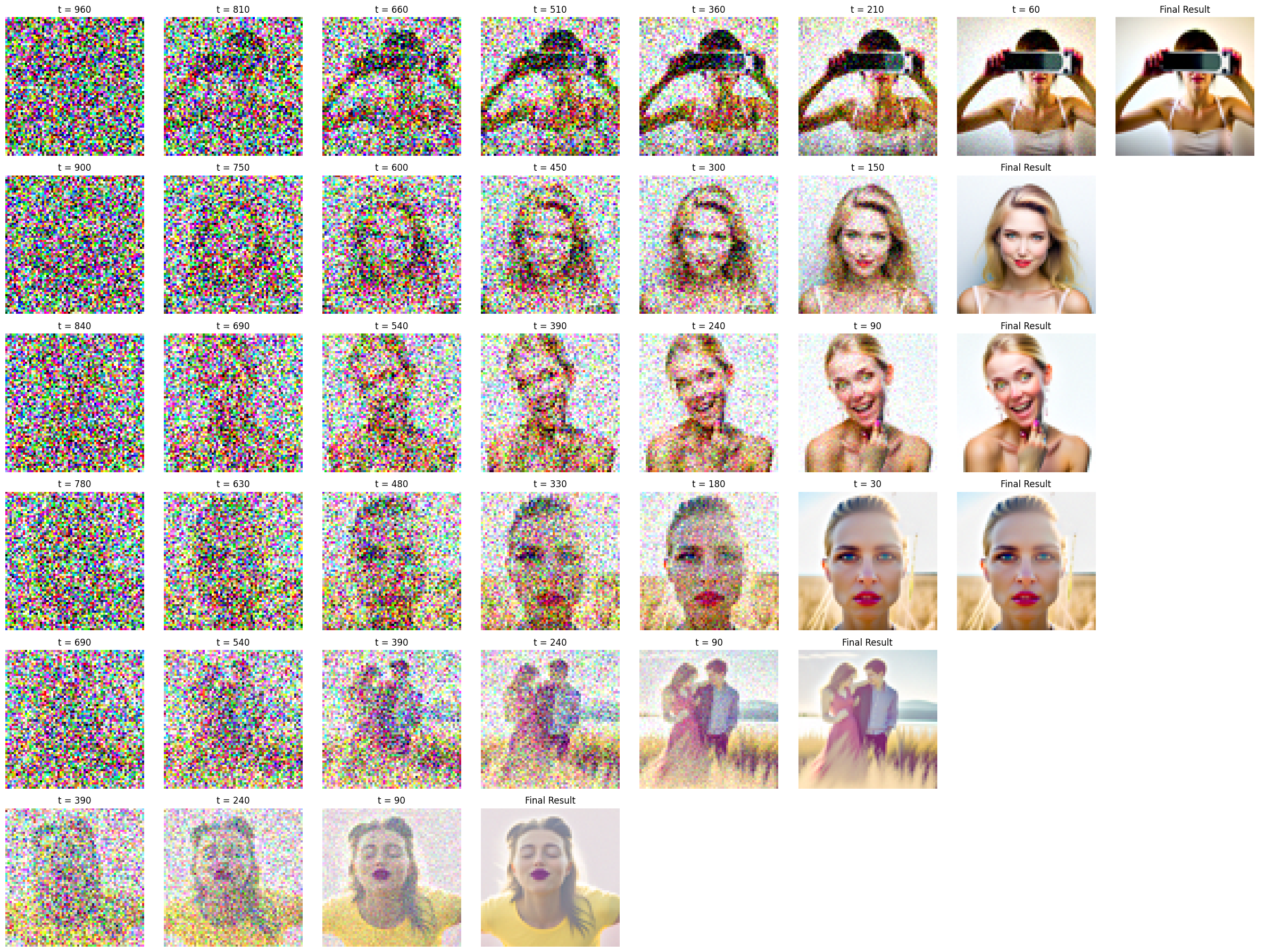
Here are two more test images, Oski and Guinness Beer.

Let's run the same process as above on the image of Oski.

i=1

i=3

i=5

i=7

i=10

i=20

Now, let's try the image of the Guinness beer:

i=1

i=3

i=5

i=7

i=10

i=20

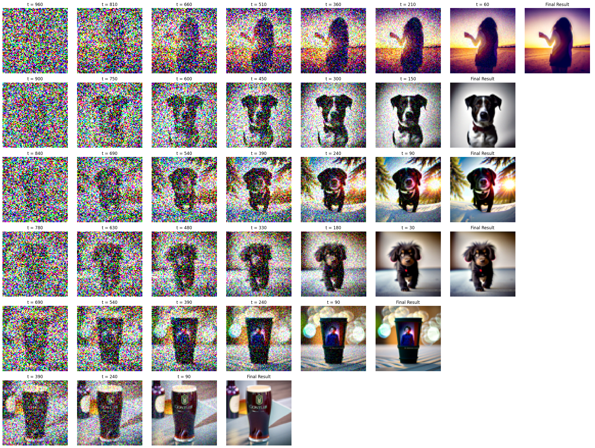
Note that my selected test images did not have as nice of a progression effect as the campanile because the pictures I chose were not as recognizable.

1.7.1 Editing Hand-Drawn and Web Images

In this part, we will experiment with how we can apply the ideas from the SDEdit paper to convert our hand-drawn pictures into realistic images! We will be applying the same exact process above.

For the non-realistic web-image, I will be using a picture of Po from Kung Fu Panda because he is super beast.

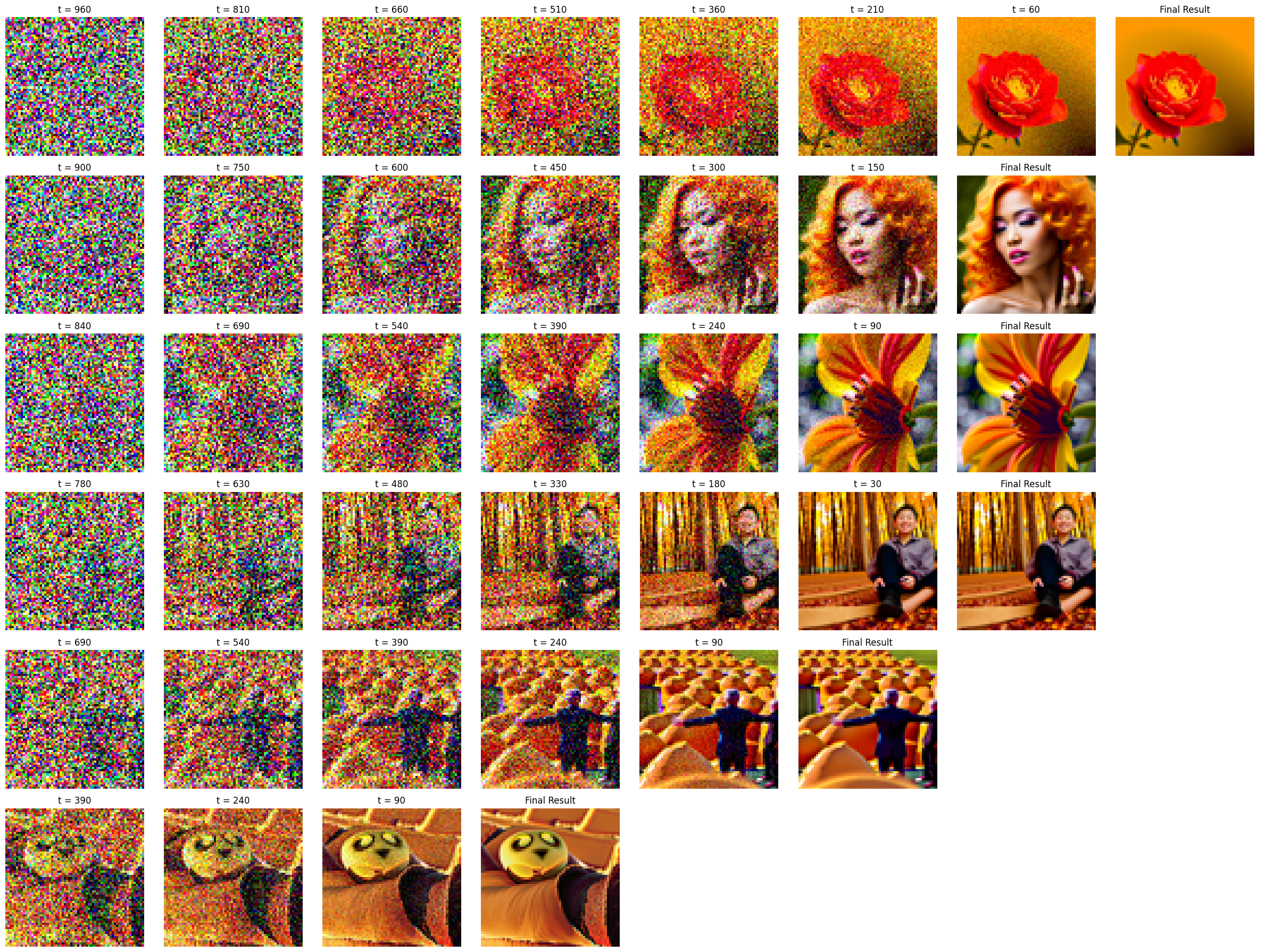
Here is the process with starting index values of [1, 3, 5, 7, 10, 20], where the first image is at t=1 and the last image is at t=20.

Next, we will apply the same process to drawn images. Here is my beautiful drawn image of a mountain with some clouds in the background and a tree in the foreground.

Below is the iterative process of denoising each noisy image:

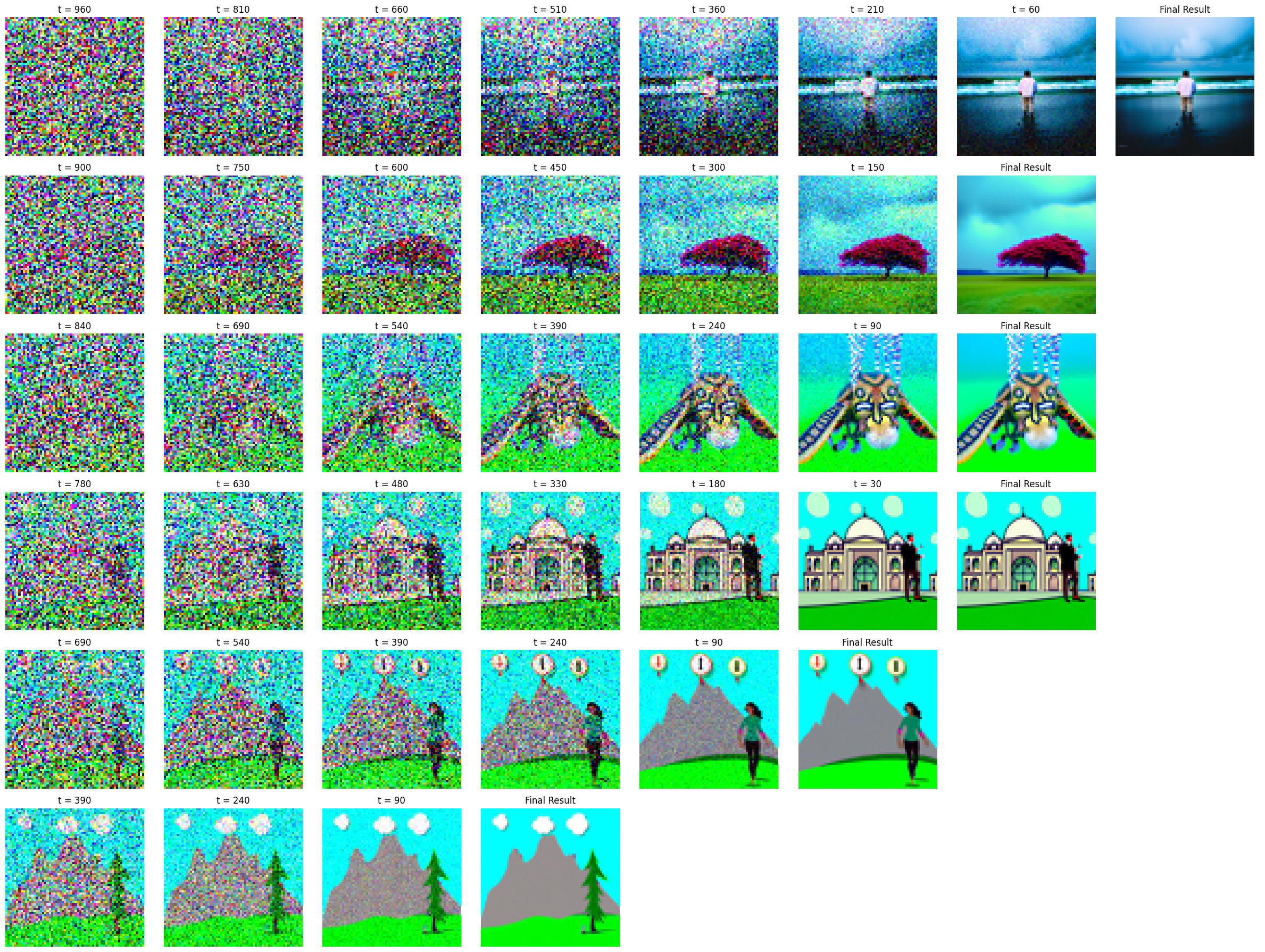
Here are the final results:

For the second drawing, I drew a sail boat in the ocean, pictured below.

Here's the progression of the model:

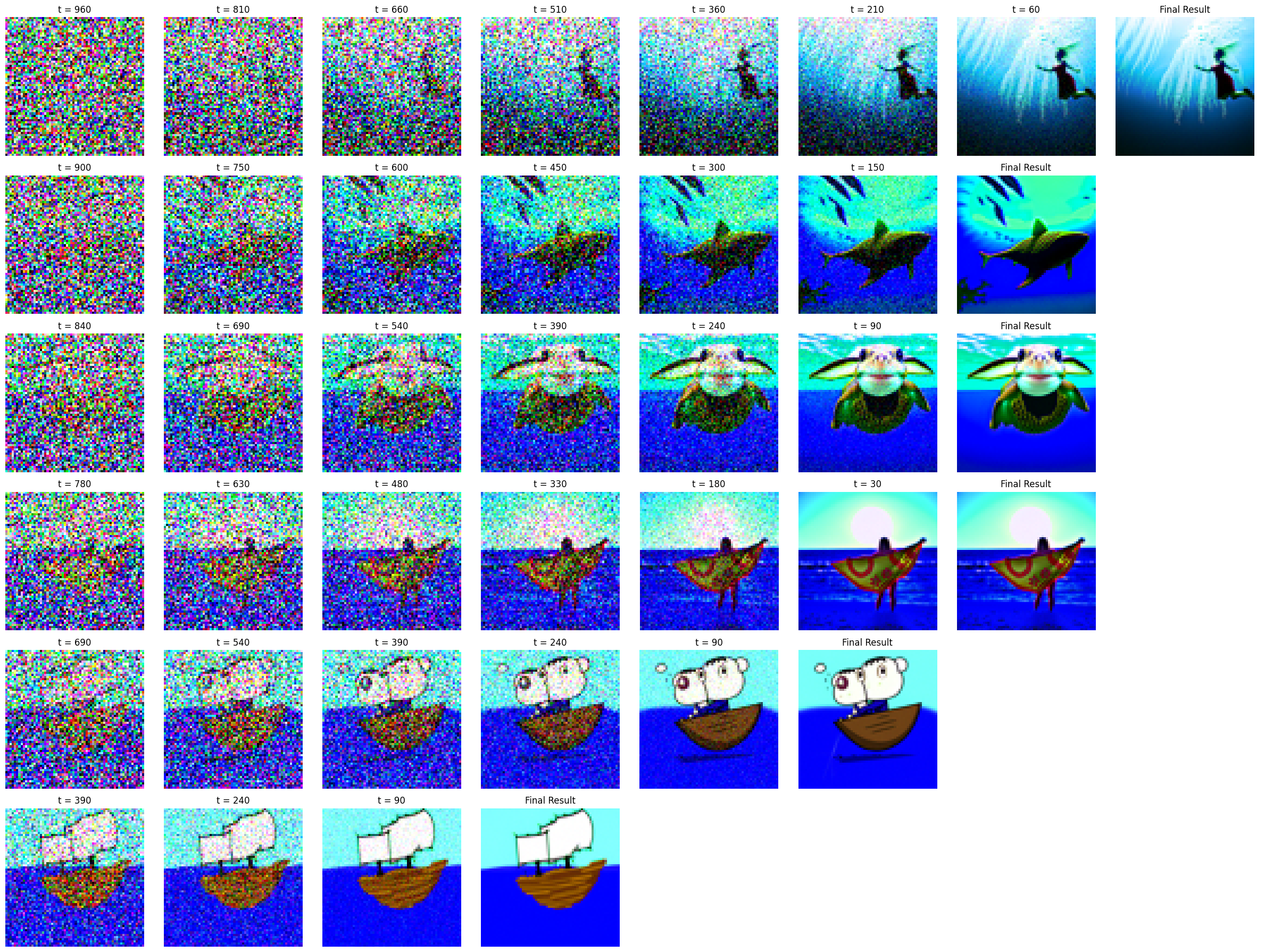
Here are the final result images:

1.7.2 Inpainting

In this part, we will implement inpainting, where we use a diffusion model to fill a blank portion of an image. Suppose we have a mask that is set to one in areas the diffusion model will fill and zero where we want to retain the original image. To do this, we apply the following equation during the denoising process:

$x_t \leftarrow \textbf{m} x_t + (1 - \textbf{m}) \text{forward}(x_{orig}, t)$

Here is an example with the Campanile:

Original Image

Image Mask

Section that will be replaced

Original Image of UC Berkeley's campus

Mask

Section of image that will be masked out

Original Image

Mask

Section of image that will be masked out

1.7.3 Text-Conditioned Image-to-image Translation

Previously, we have been using the embedding of the prompt "a high quality photo" as the text embedding for the diffusion model. In this part, I will demonstrate how changing this prompt affects the generation of the model. Similar to previous parts, we will show the generation of a test image starting at various starting indices of noise levels, ranging from [1, 3, 5, 7, 10, 20].

Here is what happens when I apply the prompt "A rocket ship" to the photo of the Campanile.

Note: First progression image shows i_start=1 and the last shows i_start=20

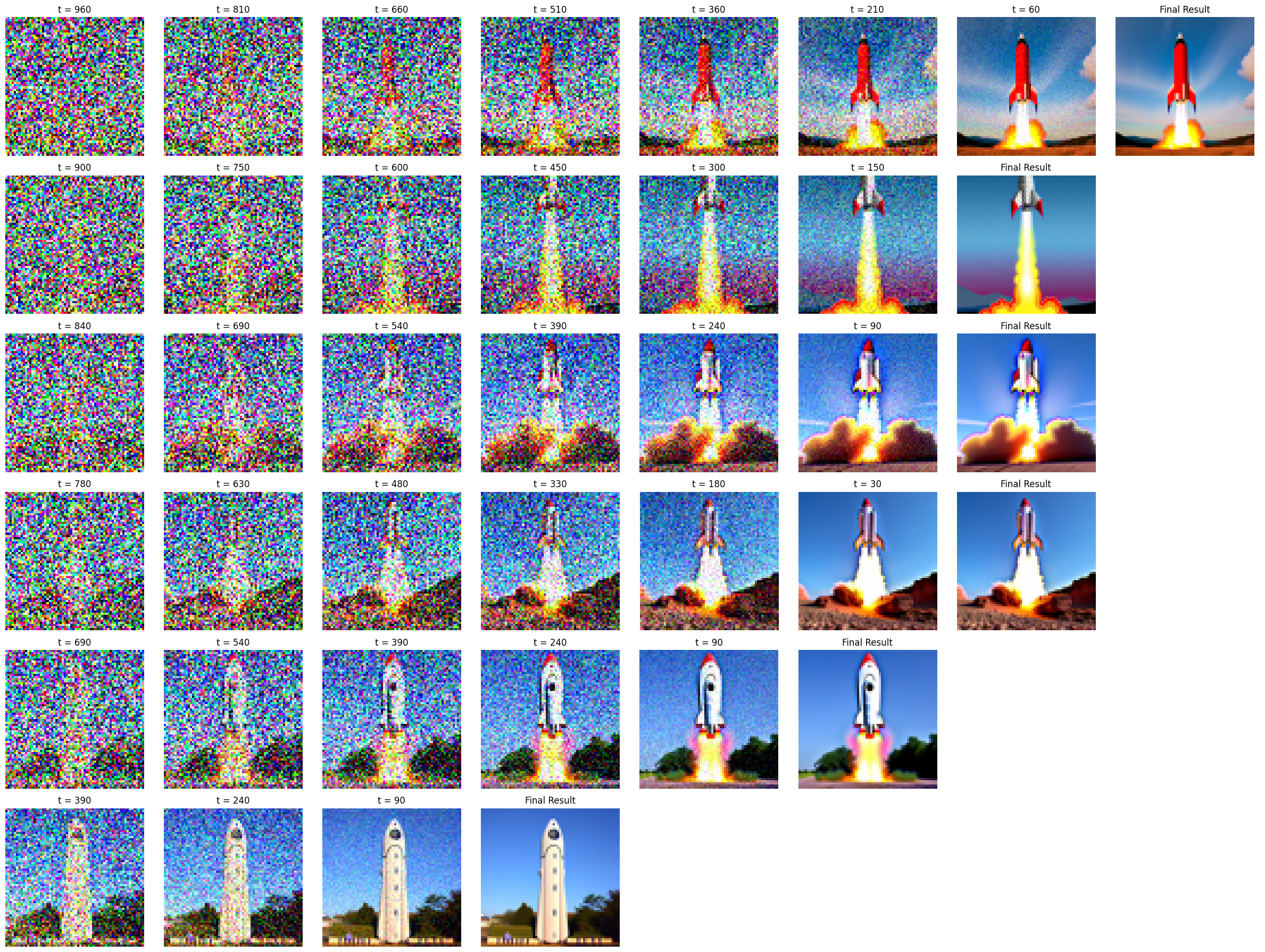
Here are the results: (Top to bottom, left to right with i_start values of [1, 3, 5, 7, 10, 20])

Here is what happens when I apply the prompt "a photo of a hipster barista" to the image of Mark Zuckerberg.

Note: First progression image shows i_start=1 and the last shows i_start=20

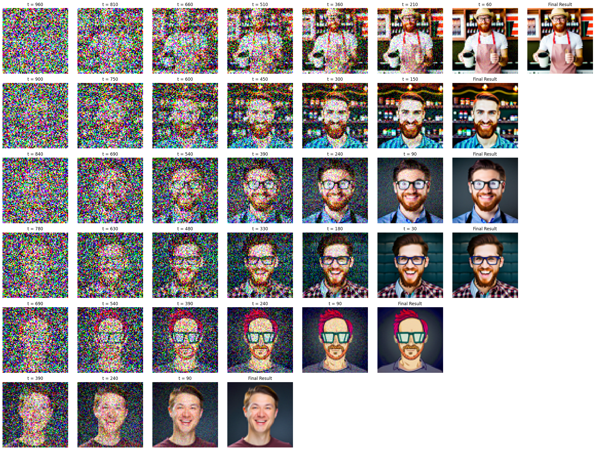
Here are the results: (Top to bottom, left to right with i_start values of [1, 3, 5, 7, 10, 20])

Here is what happens when I apply the prompt "a photo of the amalfi coast" to the image of UC Berkeley's campus.

Note: First progression image shows i_start=1 and the last shows i_start=20

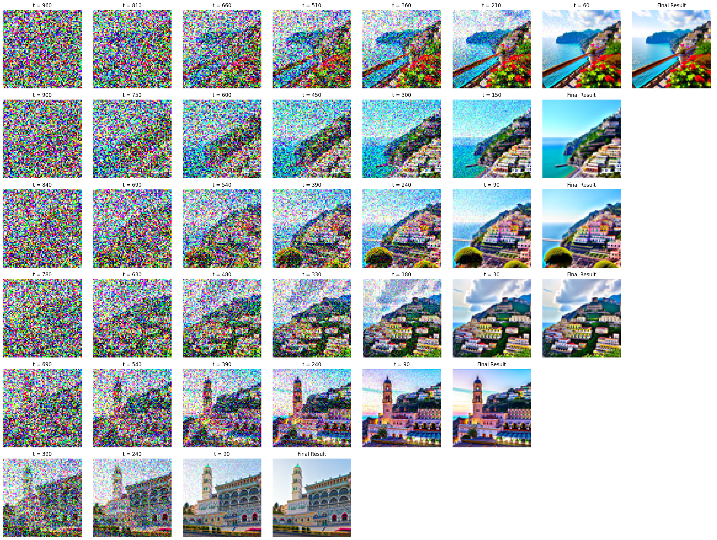
Here are the results: (Top to bottom, left to right with i_start values of [1, 3, 5, 7, 10, 20])

1.8 Visual Anagrams

In this part, we will alter the predicted noise to be a linear combination of the denoising result of two different prompts and flipping one of the predicted images upside-down to create a neat combination. To do this, I implement the following equations:

$\epsilon_1 = \text{UNet}(x_t, t, p_1)$

$\epsilon_2 = \text{flip}(\text{UNet}(\text{flip}(x_t), t, p_2))$

$\epsilon = (\epsilon_1 + \epsilon_2) / 2$

Here is an example of a image created using this process:

The image above appears to be of an old man, but if you look at it upside down, it's also an image of people around a campfire. To create this image, I biased the weight given to the "an oil painting of an old man" prompt by 75% and the "an oil painting of people around a campfire" prompt by 25%. This was done because the output was only producing upside-down images of people around campfires with no hints of an old man in the image.

Here's a visual anagram of "a photo of a dog" combined with "a photo of the amalfi coast":

Finally, here's a visual anagram of "a lithograph of waterfalls" and "a lithograph of a skull":

1.10 Hybrid Images

In this part, I create another function for image generation called make_hybrids which takes in two prompts and combines them to create a hybrid image. To do this, I apply a low-pass filter to the predicted noise outputted from the U-Net conditioned on the first prompt. Then, I apply a high-pass filter to the predicted noise conditioned using the second prompt. Finally, I simply add the noise together and continue the process as normal. As for the predicted variances, I applied the same low/high pass filters respectively and summed the terms together.

Note that in my implementation, I had to modify the values of sigma for some of the generations. For instance, in the example below of the dog and rocket ship, my function would only generate a rocket ship and no dog. Thus, by increasing sigma, I gave more weight to the low frequency

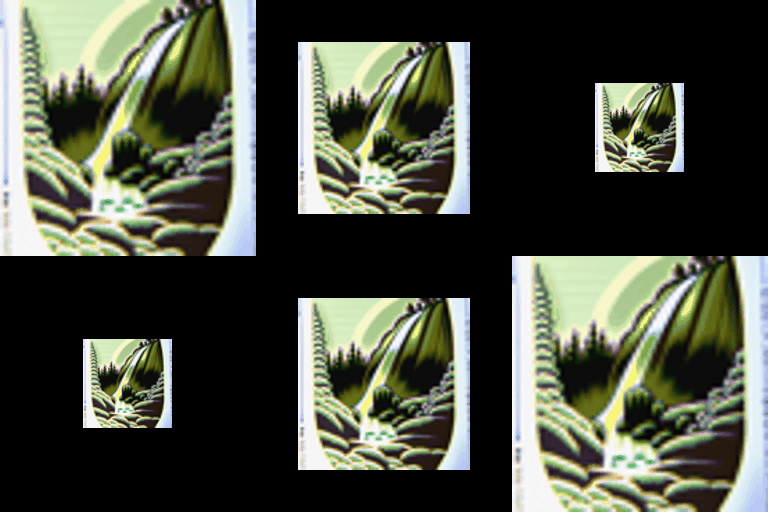
I also created a really neat function that zooms in/out of the image to demonstrate this effect.

Here is an example using the low-pass prompt "a lithography of a skull" and the high-pass prompt "a lithography of waterfalls".

Next up, here is an image generated using the low-pass prompt "a rocket ship" and the high-pass prompt "a photo of a dog".

Result Image

Up close, it shows a dog wearing a red shirt

From afar, it shows a rocket ready to launch in the desert

During my attempts to generate the above image, I got this funny result of a dog-rocket

Below is another example of a hybrid image, where from far away, the image looks like "a rocket ship" and from up close, the image appears to be a "a man wearing a hat”.

Project 5B: Diffusion Models from Scratch!

In Part B of this project, I built a diffusion model from scratch. But before that, I trained a U-net to denoise noisy images from the MNIST dataset.

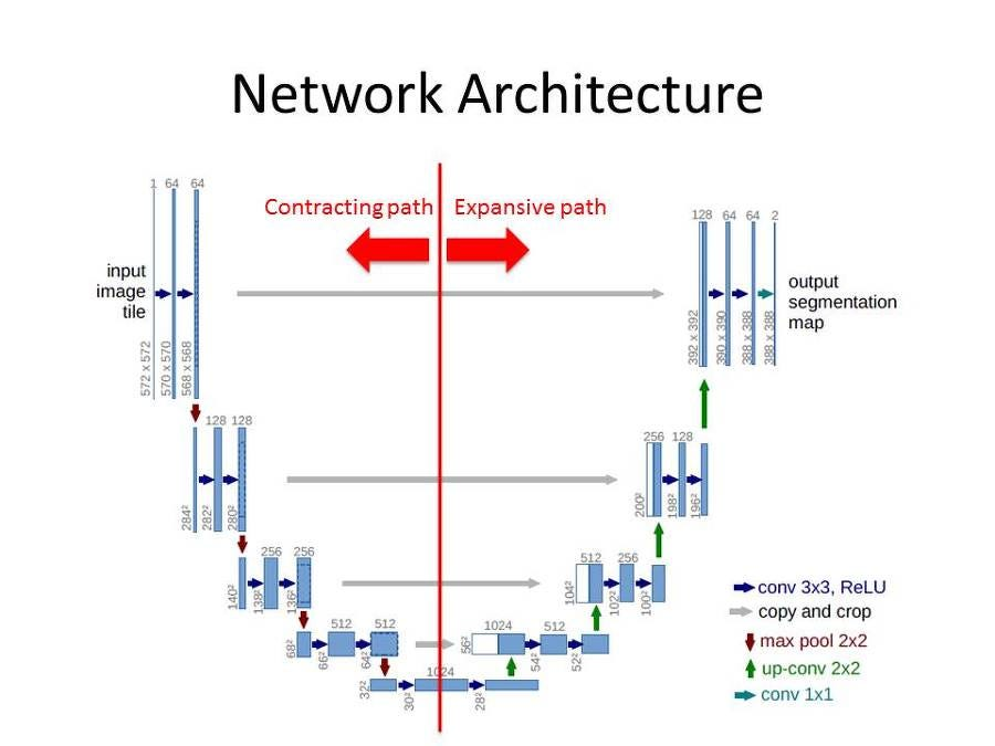
Below is an image that highlights the overall U-net architecture:

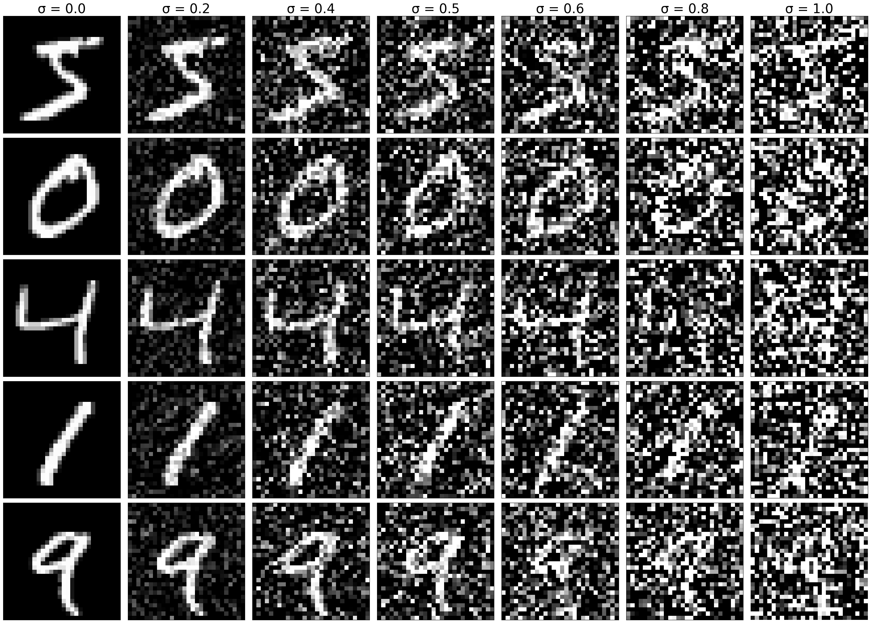
To demonstrate how adding noise changes the appearance of the original image, I created this figure below that displays the effects of applying varying levels of noise to an image where $\sigma=[0.0, 0.2, 0.4, 0.5, 0.6, 0.8, 1.0]$

1.2.1 Training

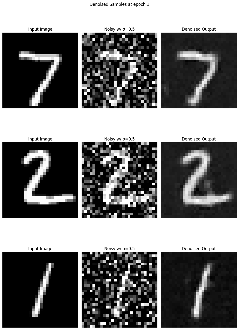
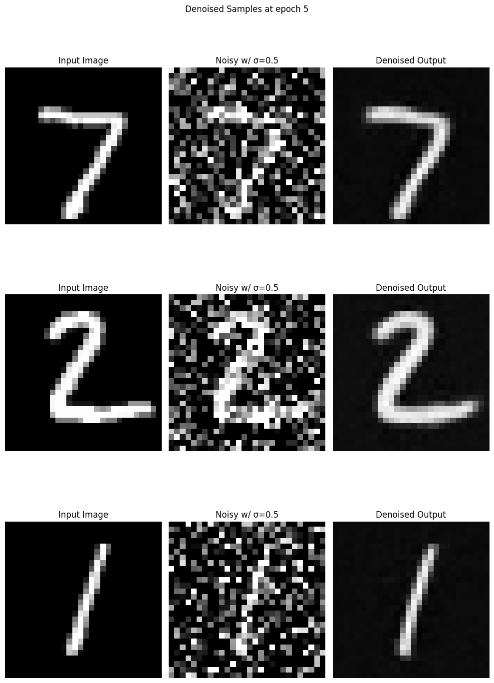
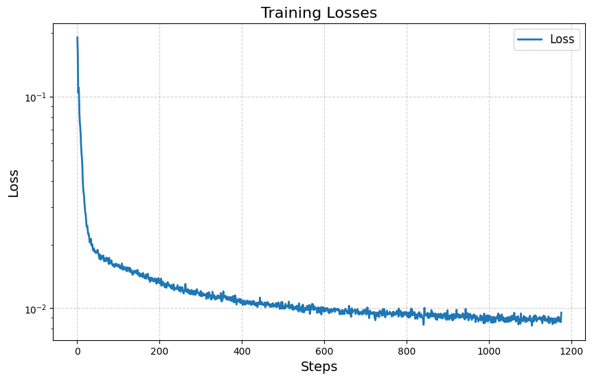
To train the model, I utilized the MNIST dataset and passed a noisy image with $\sigma=0.5$ to the model to denoise. I also created some charts showing how the predicted output of the model at different epochs.

Here are some figures of how my model learns during training over 5 epochs, starting with epoch 1 and ending in epoch 5.

Here is the training loss curve:

1.2.2 Out-of-Distribution Testing

Here is how my trained model handles out-of-distribution examples, where I test how it behaves when receiving images with sigma values $\sigma=[0.0, 0.2, 0.4, 0.5, 0.6, 0.8, 1.0]$

As you can see, the model generalizes very well in less noisy photos, but as the noise increases, the model fails to generate anything meaningful. I will address this in Part 2.

Part 2: Training a Diffusion Model

In Part 2, I prime the model on the current timestep in the denoising process

2.1 Adding Time Conditioning to UNet

In this section, I add time conditioning to my model by modifying the model's architecture and generating a random t during training, passing it to the model. This way, the model learns to denoises $\dfrac{1}{T}$ of the noise in the image based on the current t-value, such that when this process is iteratively applied T times, the model can generate a brand new, unnoisy image!

2.2 Training the UNet

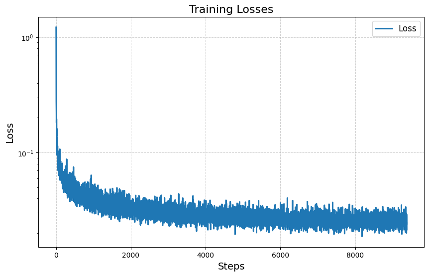
In my implementation, I trained the model over 20 epochs with initial learning rate 1e-3 and a learning rate decay rate $\gamma=0.5**(1/20)$. I also use batch size 128. I used 64 hidden layers.

Here is the training loss:

2.3 Sampling from the UNet

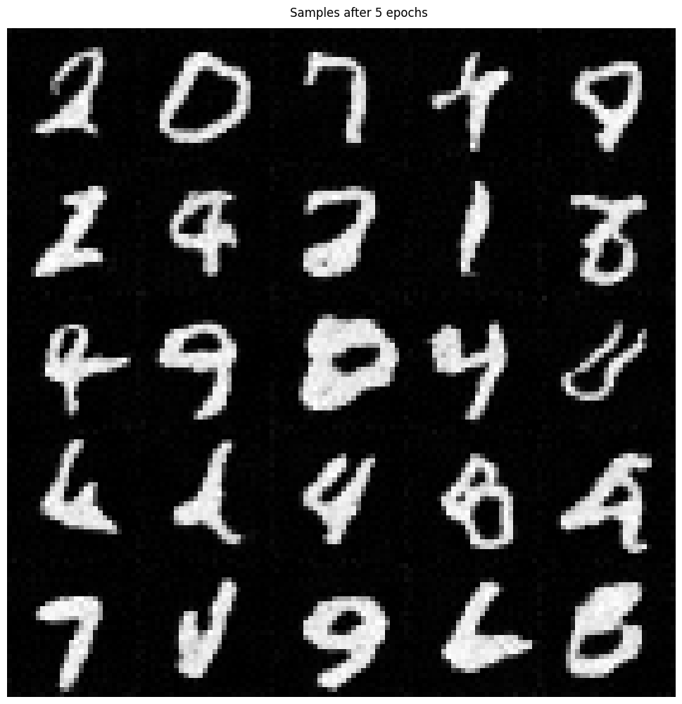
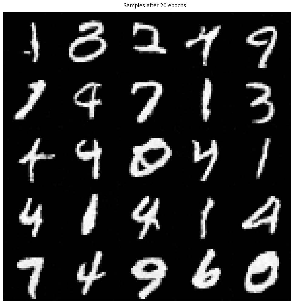
Below are some sample diffusion generations taken at different epochs during the training process.

Here are the results at epoch 5:

Here are the final results at epoch 20:

2.4 Adding Class-Conditioning to UNet

In the previous section, you might notice that there was no way to instruct the model on which number to generate. Given the initial noisy image, the model generated whichever number it felt was most optimal.

In this section, I address this issue by adding class conditioning to my model architecture. This way the model will be forced to generate an image of whatever class (in this case, digit 0-9) it is conditioned on during the sampling process.

To do this, I add two fully connected Linear blocks to my model, where I respectively multiply the result with the unflatten operation's result and the upBlock operation's result. I still keep the time-conditioning blocks from previous sections, as these are crucial for the diffusion process.

I trained my model using a batch size of 128 and an initial learning rate of 1e-3 with an exponential learning rate scheduler. I also used 64 hidden layers and a probability of not including the conditioned class of 0.1. This probability hyperparameter helps teach the model to generate basic images of any digit so it can then learn which digit is which.

Here is the result of my training after 20 epochs.

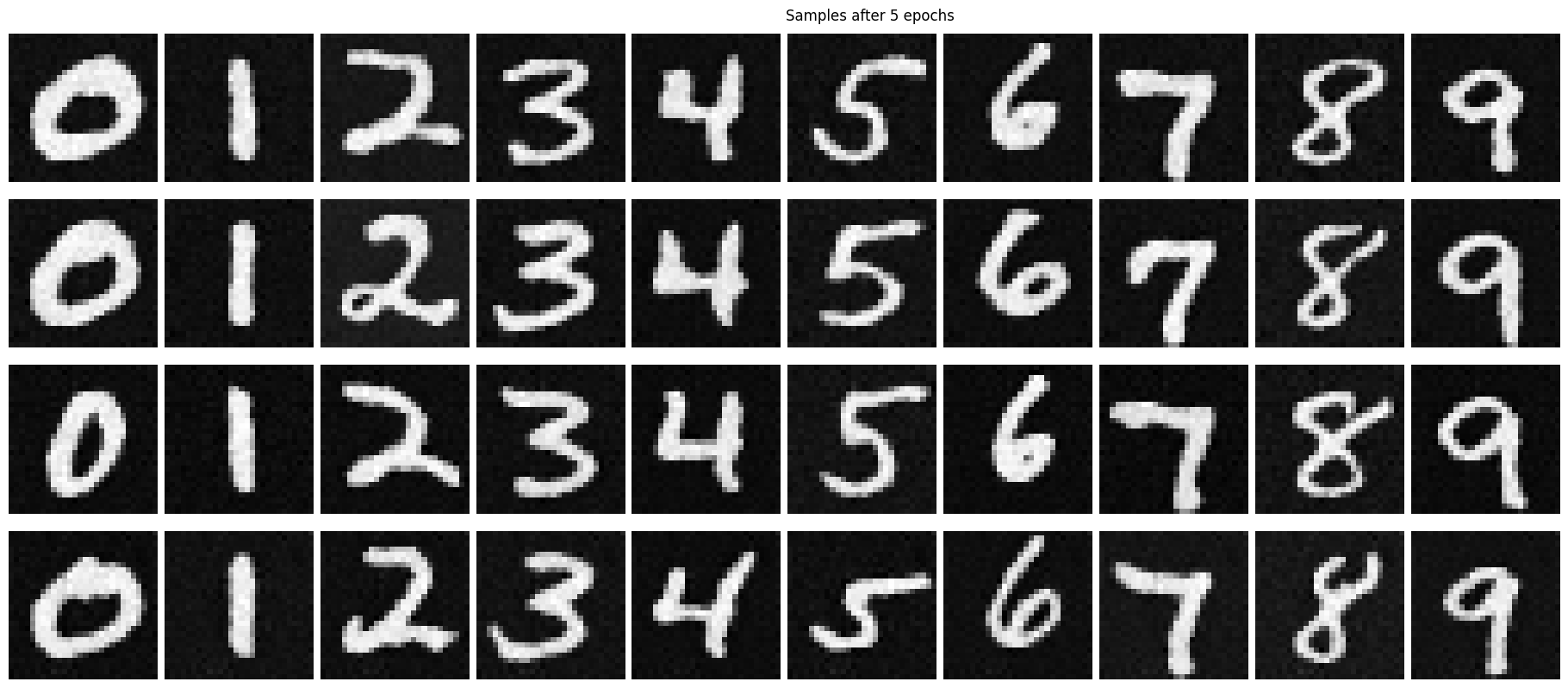
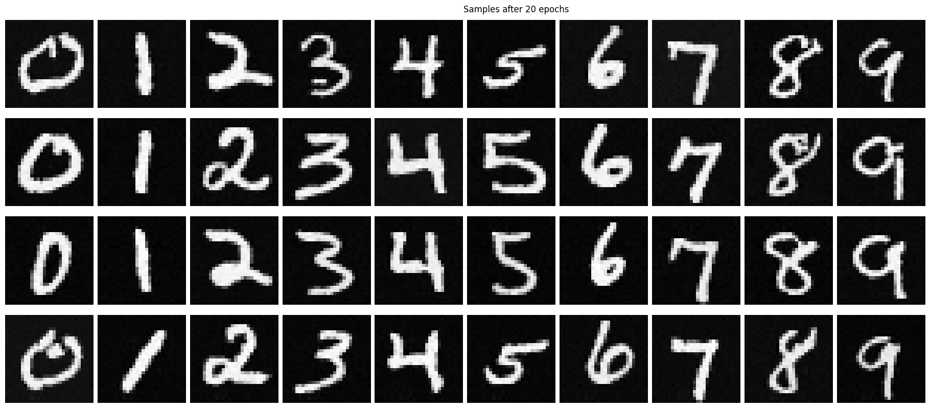
2.5 Sampling from the Class-Conditioned UNet

Now that I can condition which class I want my diffusion model to generate, I can create an array of numbers from zero to nine.

Here is what sampling looks like after five training epochs:

Here is what sampling looks like after twenty training epochs:

Side-Note

I just wanted to say thank you to the course staff for creating this project. It was fascinating to learn how intuitive diffusion models are, and I had a blast working on this project :)